Neural networks

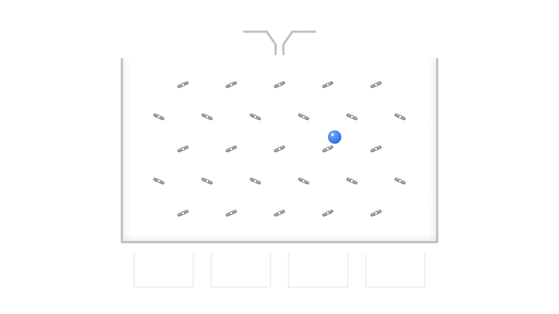
Drop a ball into a Plinko board and it bounces from peg to peg. Where will it land? That uncertainty is part of the game.

But what if we wanted a particular result? Imagine pegs we could adjust to guide the ball toward a chosen exit. Then raise the challenge: send different shapes to different bins—a ball to one, a cube to another, a prism to a third, and even a toy dinosaur to a bin of its own.

How would we find the right peg settings? We could drop a shape, see where it lands, and adjust the pegs whenever it goes to the wrong place, then keep trying other shapes until each one reaches its intended exit.

A board adjusted to sort those shapes is like a trained neural network: it takes an input and produces the intended output. The repeated process of trying, checking, and adjusting the settings is what we mean by learning. A real neural network, of course, works with numbers and connected calculations rather than pegs and bouncing objects.

Look closely at any one of the neurons in that network and you find, at its core, simple math. Start with a very simplified neuron. Its input is a number between 0 and 1, and we want it to output 0 when the input is below 0.5, and 1 when the input is 0.5 or above.

The neuron multiplies the input by a weight, then rounds the result to 0 or 1. What weight would make this work?

A weight of 1 works, because it leaves the input unchanged: 0.4 × 1 stays 0.4 and rounds to 0, while 0.5 × 1 stays 0.5 and rounds to 1. The rest of this chapter builds on this simple example.

Give our neuron a real job: controlling a sound-activated light. Imagine a microphone measuring the sound level in a room, represented as a number between 0 (silence) and 1 (very loud). The sound level is the neuron’s input, and its output controls the light: 1 means on, 0 means off.

Inside, the neuron multiplies the sound level by its weight; the weight controls how strongly the sound affects the score. Because the light needs a plain yes or no, we round the score at the output: below 0.5 rounds to 0 (light off), and 0.5 or above rounds to 1 (light on). That rounding is our choice for this job, not part of every network; different jobs attach different finishing steps to the output.

The goal is to have the light on when the sound level is 0.3 or higher, and off below that. Try the simplest weight, 1, which passes the sound level straight through. A sound level of 0.4 is above 0.3, so we want the light on. But 0.4 × 1 is 0.4, which rounds down to 0, so the light stays off. The neuron needs a different weight. What weight would connect the goal’s threshold of 0.3 with the neuron’s cutoff of 0.5?

Choosing a weight by hand works when there is only one weight, but we want a method a machine can follow. We can borrow the one we imagined for the Plinko board: try, check, adjust.

First, gather practice sounds: a handful of levels between 0 and 1, each paired with the answer we want (on at 0.3 or higher, off below). Start at weight 1. The first sound, 0.4, should turn the light on, but it stays off: the score came out too low, so we nudge the weight up. The next sound, 0.2, should leave the light off, and it does; correct answers get no nudge. When the light comes on but shouldn’t, the weight is too sensitive, so we nudge it down.

This loop—try a sound, check the answer, nudge the weight—is what training means. Step through the run below, one sound and one nudge at a time: the nudges shrink, the misses fade, and the weight settles at 1.67. Then comes the real test: fresh sounds it never practiced on.

With a single weight, simple algebra could have handed us the answer directly. We took the long way on purpose. Real networks have millions or even billions of weights, and no formula solves for them all at once; the try-check-adjust loop, one nudge at a time, scales to any size.

The light was a very small machine: one input, one weight, one answer. Yet that tiny piece of math is the seed everything else grows from.

The light responds to a single number, the sound level. Recognizing a spoken word or a picture takes many more: an image, for example, is usually described by one number for each pixel’s brightness. So the neuron grows. Each input gets its own weight, and the neuron adds all the weighted values into one score. There are more inputs and more weights, but still one output: the neuron’s response, called its activation.

The neuron below has three inputs. Change its weights and see how the total responds. It also adds a number of its own, a bias, which the next page explores. Later, this same neuron becomes part of the tiny network we use to examine learning up close.

A typical neuron also adds one number of its own: the bias. To see why, consider what happens when every input is zero. Without a bias, zero in always means zero out, because anything times zero is zero.

But zero is not an empty message. Silence tells you something about a room, and a dark corner tells you something about a picture; sometimes the right response to zero isn’t zero. The bias is the neuron’s own starting number: it sets where the total starts, even when every input is zero. The weights control how the total changes, and the bias lets it start above or below zero. Training adjusts both: every weight and every bias.

The bias can also move the decision point itself. For the light, we reached the goal by scaling, with a weight of about 1.67. A bias offers another route: keep the weight at 1, add a bias of −0.3, and move the cutoff too—instead of rounding at 0.5, the light now turns on when the score is zero or above. The score becomes simply the sound level minus 0.3, which crosses zero exactly at the goal. The result is the same, but instead of scaling the sound to meet a fixed cutoff, the bias and the new cutoff together shift where the decision happens. (That zero cutoff is in fact the standard arrangement: real neurons fold the threshold into the bias and compare at zero.)

So far, the recipe reads: weigh, add, bias.

A single neuron makes one simple call. Recognizing anything real takes many small decisions working together toward a bigger one, so we need more neurons, and there are two directions in which to add them.

We can add companions: more neurons reading the same inputs side by side, each with its own weights and each making its own call. A group like this forms a layer. Or we can grow in the other direction, adding a second layer that reads not the inputs but the first layer’s answers, so that decisions build on decisions. Step through the stages below.

For stacked layers to add anything, the network must be nonlinear. To see why, notice that everything our neuron has done so far (multiply by a weight, add the bias) is a linear equation: a steady change in the input gives a steady change in the output, so a graph of output against input is always a straight line. Linear equations are very good at drawing lines, and lines are all they can ever draw.

Stacking them, so that each equation’s output feeds the next, doesn’t change this. Follow the chain below. The first equation turns x into y₁; the second takes y₁ as its input and produces y₂; the third does the same with y₂. The tinted pills mark each shared value, produced by one equation and used by the next. Each stage tilts, shifts, or flips the line, but what comes out is always another line. In fact, you can multiply the whole chain out into a single equation of the same form. Ten layers or a hundred, the result is still one line, and a line can never trace anything more.

Since stacking straight lines can never escape the line, we change the neuron itself. At the very end of each neuron we add one small nonlinear rule, a bend that acts as a gatekeeper. A total of zero or less becomes an activation of zero, so the neuron stays silent; a positive total passes forward at full strength. So 3.2 stays 3.2 and 1.3 stays 1.3, while −0.5 becomes 0.

Drawn as a graph, the rule is the bend: flat at zero, then a straight climb. As math, it is one short expression: activation = max(0, total), the larger of zero and the total. The rule is called ReLU, short for rectified linear unit, and is usually written ReLU(x) = max(0, x): keep the positives, zero out the rest. It is the most common of many such rules.

Try it on our three-input neuron: move its bias and see its total slide along the bend.

With nonlinear pieces, we can rebuild. Put two bends side by side and add them, and you get a V; our temperature example did exactly that, with one ReLU measuring how much too warm and the other how much too cold. A few more bends make a peak, then a wave—already far more than any line could draw.

Adding bends side by side is what width gives us: more neurons in one layer, their outputs combined by the next. Stacking goes further, because each new layer can bend what the last one drew. A new layer reads the finished curve, lowers it with its bias, and bends it again: lower our wave by 0.2 and bend it, and the zigzag becomes two separate peaks. Keep going, and you can trace even the outline of a face. Networks built this way can represent truly complex patterns.

That is what nonlinearity buys: layers that don’t collapse into one, each building on the shapes made by the layer before. Different inputs activate different mixes of neurons, and because layers build on layers, a network can learn in stages. Imagine reading a picture that way: dots gather into edges, edges into a circle, a circle becomes an eye, eyes become a face, each stage reusing the one before. A single layer working alone, with no stages to lean on, would need a separate rule for every face it might ever meet—long ears, short ears, eyes open, eyes closed—an endless catalog, one giant layer wide. A deep network learns its pieces once and reuses them everywhere.

That is why nearly every neuron ends with a nonlinear rule. Modern networks add other moves on top of this recipe, but these four steps remain its heart. One complete neuron: weigh, add, bias, bend.

Connecting layers involves choices. Keep the same four inputs and the same two outputs; the hidden layers between them are ours to design. We could put three neurons in one hidden layer, or five—a wider layer, with more neurons calculating from the same inputs. Or we could stack three hidden layers of three neurons each—a deeper network, with more stages, where each layer works with the results of the one before.

The number of neurons in a layer is its width; the number of successive layers is the network’s depth. Networks with several processing layers like this are what “deep learning” refers to. Either way, the inputs and outputs are unchanged. And neither choice promises better answers: which arrangement works better is something you measure, not assume.

With all the pieces in hand, we can build a real neural network with an actual job: reading handwritten digits.

People write the digits 0 through 9, and every one comes out a little different. We want a machine that looks at one and says which digit it is. We use real images from a collection called MNIST: 70,000 handwritten examples that have been used to teach machines for decades. To a machine, each image is a grid of 28 × 28 pixels—784 small squares, each holding one number, its brightness, scaled from 0 for black to 1 for white.

That is exactly the kind of input our neuron takes: numbers between 0 and 1, only now there are 784 of them, one per pixel. So the image fixes the input side of the network. What comes after the inputs is a choice.

For the middle, we choose one hidden layer of 32 neurons. That is not a magic number; it is a design choice. Each neuron reads all 784 pixels through its own set of weights—784 weights per neuron—and runs the recipe we know: weigh, add, bias, bend.

Unlike our light switch, these neurons don’t answer simply on or off. Each outputs a number saying how strongly it responded to what it saw, so the 32 neurons produce 32 responses for the next layer to work with. Their weights and biases are parameters, numbers that training learns; the values shown come from our already-trained network.

The question itself decides the output side: ten digits, so ten outputs, one score per digit. Each output is a neuron of its own, with its own weights, reading all 32 hidden responses.

Their scores then get a finishing step. It isn’t the rounding we used for the light: the ten scores become probabilities that always add up to 100%, and the highest probability wins. That step is called softmax; we look inside it when we study learning.

Before training, a network’s probabilities are essentially arbitrary. Training aims to push the correct digit’s probability toward 100%, and every other digit’s toward zero, by adjusting the weights and biases. How were all those thousands of weights and biases set? With the same loop we ran for the light, done by machine across every weight at once: show the network a digit, check the probability it gives the correct answer, then adjust every weight and bias a little, nudging that probability up and the others down. We ran that loop over 60,000 training images, five passes in all. After training, the network gives the real handwritten 7 shown first below a probability of 98.6%, putting 7 on top.

We trained a second network the same way, this time with two hidden layers: 64 neurons, then 32. The 784 inputs and ten digit outputs stayed the same. Then came the real test: 10,000 images that neither network had seen during training.

The one-hidden-layer network identified 95.58% of them correctly (9,558 of 10,000); the two-hidden-layer network reached 96.35%, 77 more. In this experiment the bigger network won. But it got deeper and wider at the same time, so we can’t credit depth alone, and one measurement on one problem is no promise that bigger always wins.

To see how training actually works, we need a network small enough that every number inside it is visible. So here is a tiny, untrained version of the digit network: imagine the image squeezed down to just three numbers instead of 784 pixels, feeding two hidden neurons (the three-input neurons from the basics) and the same ten outputs. We give it the same test as before: the right answer is 7.

Each of the ten output neurons produces a score, and softmax uses all ten together to produce ten probabilities that add up to 100%; a larger score gets a larger share. Untrained, our network gives its largest share to 3, for no reason at all. Before training, a network’s weights and biases are just starting numbers. In practice they are picked at random; ours were chosen by hand for this lesson. Whatever they are, the probabilities land somewhere, and ours landed on 3. The right answer, 7, gets only about 9.3%.

To improve the network step by step, we first need a single number that says how wrong it is on this example. That number is called the loss.

The loss should behave in a particular way. If the network gave 7 everything (100%, and zero to every other digit), it would be perfectly right, so the loss should be zero. The smaller 7’s probability gets, the more wrong the network is, so the larger the loss should grow: giving 7 a 90% probability is better than giving it 10%.

A very common choice, and the one we use, is the negative logarithm of the probability. It rises slowly at first, then shoots up steeply as the probability heads toward zero—exactly the behavior we want. This rule is called cross-entropy loss, and our 9.3% gives a loss of 2.37. The smaller the cross-entropy, the closer the network’s outputs are to what we expected. Other jobs use other loss functions; this is the one for our example.

Which change would make the loss smaller? Start with the simplest experiment: nudge one weight and see what happens. Take the weight from input 2 (value 0.8) into hidden neuron 2 and raise it by 0.05. The change ripples forward through the network: that neuron’s output shifts by 0.04, the score for 7 by 0.016, and the loss falls by 0.0065.

That experiment tells us two things: the direction (raising this weight helps) and the strength (how hard the loss reacts when this weight moves). Together, direction and strength make up this weight’s slope. That is all a slope is: which way helps, and how much it matters.

The curve below shows the same idea for a different weight, the one from neuron 1 to digit 7. With every other weight and bias held fixed, it plots the loss (vertically) at many values of this one weight (horizontally); the dot marks the current setting.

We need the same answer for every weight and bias—all 38 of them. In our tiny network we could nudge them one at a time and rerun the network 38 times. But our digit network has 25,450 weights and biases, and its training took 2,345 updates; nudging one at a time would mean rerunning the whole network nearly 60 million times. Modern networks have billions of weights. One at a time is hopeless. Instead, a method called backpropagation gets every answer in one backward pass. To see how it works, we need one small idea first.

Take the simplest kind of neuron: one weight, one input, one bias. Written as plain math: weight × input + bias = output.

Ask one question: if the weight grew by exactly 1, how much would the output change? That question—how much the output changes per unit of change in one part—is what a derivative answers. It is the slope again, under its formal name: the derivative of the output with respect to that part.

Try it. Say the weight is 2, the input is 5, and the bias is 1, so the output is 2 × 5 + 1 = 11. Raise the weight to 3, and the output becomes 3 × 5 + 1 = 16. It moved by 5, which is no accident: 5 is the input. Each extra unit of weight adds one input’s worth to the output, so the derivative of the output with respect to the weight is the input.

The same test works for the other two parts. Raise the bias from 1 to 2, and 11 becomes 12: the output moves by exactly 1, so the bias’s derivative is always 1. Raise the input from 5 to 6, and 11 becomes 13: the output moves by 2, which is the weight. So the input’s derivative is the weight.

That is how simple calculating a derivative can be. Keep the shape of the idea: the derivative of one thing with respect to another tells us how changing the second changes the first. Its size matters as much as its sign: a bigger derivative means the same small nudge makes a bigger change.

Put two of these neurons in a row. The first computes w₁ × x₁ + b₁, and its output is x₂. The second reads that output and computes w₂ × x₂ + b₂; its output, x₃, is the network’s answer. To score the answer we need a loss, and here we use a simpler one than our digit network does: half the squared difference between the expected answer and the actual one, ½(expected − x₃)².

Run it once with x₁ = 2, w₁ = 3, b₁ = 1, w₂ = 2 and b₂ = 1. Then x₂ = 3 × 2 + 1 = 7 and x₃ = 2 × 7 + 1 = 15. We wanted 13, so the loss is ½ × (13 − 15)² = 2.

The goal is to find, for every weight and bias (w₁, b₁, w₂, b₂), which way it should move and how much it matters: the derivative of the loss with respect to each one. Backpropagation is the method that finds them all.

It starts with the only value whose formula touches the loss directly: x₃. Differentiating the loss gives the first slope: dLoss/dx₃ = x₃ − expected = 15 − 13 = +2. That is not yet a weight or a bias, but it is a foothold, and it is all we need.

The first target is w₂. Multiplying and dividing by dx₃ splits its derivative into a chain: dLoss/dw₂ = dLoss/dx₃ × dx₃/dw₂. We already have the first factor. The second comes from the derivative rule applied to equation two: a weight’s derivative is its input, x₂ = 7. So dLoss/dw₂ = 2 × 7 = 14. The bias works the same way: 2 × 1 = 2.

Equation two has one more derivative, an unusual one: with respect to its input, x₂. We can’t turn x₂ like a dial, because it is equation one’s output—and that is exactly what makes it useful. dLoss/dx₂ tells us what one unit of equation one’s output is worth to the loss. The same split-and-multiply gives 2 × w₂ = 2 × 2 = 4, and we carry that value back.

Equation one’s weight sits two steps from the loss. Split again, this time through dx₂: the carried 4 times dx₂/dw₁, which is equation one’s input, x₁ = 2, gives 8. Equation one’s bias gets 4 × 1 = 4. Nothing about equation two was needed again; the carried slope already contains everything downstream. A real nudge confirms the result: raising w₁ from 3 to 3.01 moves the loss from 2 to 2.0808, almost exactly the 8 × 0.01 = 0.08 the slope predicted.

That is the whole method. At every equation, the same two moves repeat: multiply the slope that arrived by one simple local derivative; then keep the results for that equation’s weight and bias, and hand the result for its input backward, because that input is the previous equation’s output. In the end every weight and every bias has its slope, and so knows which way to move. That is backpropagation.

Our tiny digit network does exactly what the two-equation example did, only wider. Start at the end, at the loss, and step back into the output layer. As before, there are three kinds of slopes to find: for its weights, its biases, and its inputs. The weight and bias slopes are kept, because those are this layer’s own dials. The input slopes are handed back, because those inputs are the previous layer’s outputs.

The previous layer receives its slopes just as equation one did, with one difference: each hidden neuron feeds all ten output neurons, so it collects a slope from every one of them and adds them up. Then the same two moves repeat—keep the weight and bias slopes, pass the input slopes further back—layer by layer, all the way to the start. Below, follow one output weight, then one earlier weight, including the ten paths that are added together.

One backward pass gives every weight and bias its slope at once. For our digit network’s training, that means a few thousand backward passes instead of 60 million reruns. In the tiny network, one sweep yields 38 slopes: for every weight and bias, which direction helps and how strongly. Collected together, they form the gradient, one master list of each parameter’s influence on the loss.

The result even reproduces our nudge experiment. Hidden neuron 2 collects ten slopes from the ten outputs, which add up to −0.165. Multiplying by the input its weight meets, 0.8, gives −0.13: the same slope the nudge measured (a loss change of about −0.0065 for a nudge of 0.05).

Note what backpropagation does not do. It changes nothing; it only measures. And it never sets a target: no neuron is told what its output should be. Every slope is simply a measurement: move this dial a little, and this is how the loss responds.

With the slopes in hand, we can update the network. In a single update, all 38 weights and biases move at once, each in the direction its slope says helps and in proportion to that slope: a strong slope means a bigger move, a tiny slope barely a move. This recipe is called gradient descent. A rule that turns slopes into changes is called an optimizer: backpropagation measures, and the optimizer updates.

Remember what each slope really is: the sensitivity of the loss to one weight or bias, measured while every other weight and bias stays exactly where it is. If the others then move only a little, that measurement is still dependable enough to guide this weight’s update. If they move a lot, the network has changed too much, and the measured slope may no longer reflect the true sensitivity. So the steps can’t be too big.

They can’t be too tiny either. Move by crumbs, and learning slows to a crawl; steps that small can also settle into the first shallow dip they find, with better answers waiting just past a bump they can never cross.

The step size is set by one shared dial, called the learning rate. The size of every move is the slope’s size times the learning rate, and its direction is the one that helps: new weight = old weight − learning rate × slope. Ours is 0.2, so each weight moves by one fifth of its slope. Why 0.2? No formula says so. The right learning rate is found the way everything else is found: try, check, adjust.

Take that step on our tiny digit network: every weight and bias moves at once, each by its slope times the learning rate of 0.2. Click once, and the loss falls from 2.37 to 2.08 while the probability for 7 rises from about 9.3% to 12.5%. But the answer is still 3. Better is not yet right.

That is one step of learning, and training repeats it across many examples. Try a few more clicks, or a different learning rate, and see what each step does.

So far we have improved the network on a single example, but a step that helps one example can easily hurt another. Take two training examples in our tiny network and ask each, on its own, which way a weight should move. For the weight from hidden neuron 1 to the digit-3 output, they disagree: the first example’s slope is +0.103, so it wants the weight nudged down, while the second’s is −0.371, so it wants the weight nudged up. Which one should we follow?

Both. We work out each example’s gradient separately, average them (for this weight, −0.134, so the weight goes up), and make one shared update. A group of examples handled together like this is called a batch. Recognizing handwriting requires seeing many ways of writing every digit, so we train on many labeled images grouped into small batches. Below, twelve real training images are grouped into batches; each group contributes to one shared update.

The learning rate decides how far each shared update goes. Take the same two examples and the same starting weights, and make a single update at three different rates. Their average loss starts at 2.00. At a rate of 0.05 it barely moves, to 1.97. At a rate of 2 it drops substantially, to 0.92. At a rate of 20 it does not fall at all: it explodes to 8.99. That step was so big that it overshot everything the slopes knew about.

Choose a rate below, then make one update. Every trial starts from the same weights, so the comparison isolates the effect of the step size.

Three rates tried one at a time give only three points. The curve below shows the whole range: the loss after one update at each learning rate, using the same two-example batch and the same starting weights. A small step may help only a little; a much larger one can make the loss worse.

Small steps, many examples, pass after pass: that is what training looks like in practice.

All this practice hides a trap. A network can keep improving on the images it trains on while quietly getting worse on images it has never seen: instead of learning, it starts memorizing.

Lower loss on familiar examples is useful only if it also helps with new handwriting. Return to our real 32-neuron digit model and compare an image used during training with one kept out of training; both predictions use the same learned weights. Success on new examples is called generalization.

To see the trap happen, we ran a smaller, deliberately starved experiment: only 1,024 training images, and two network sizes, one narrow (4 hidden neurons) and one wide (64).

Follow the wide network as it trains. Its training loss keeps falling, pass after pass, but its validation loss turns around and starts getting worse: the network is drifting from learning toward memorizing. By this measure, it is overfitting. The opposite problem is underfitting: a network that still struggles with its own training examples, because it has learned too little or cannot represent the needed patterns. There, more training or more neurons may help.

In that starved experiment, the validation set picked out the best moment: epoch 10 of the wide network. We took the network exactly as it was at that point and used the test set once: 88.83% correct.

That is the usual practice. We save a copy of the network at every checkpoint along the way, and when training ends, we use the one the validation set liked best—here, the network as it stood at epoch 10. Training longer was not better, so we simply set aside what came after. This is called early stopping.

To make the network genuinely better, the strongest cure is more examples. This starved network saw only 1,024 images; our 32-neuron network, trained on all 60,000, reached 95.58% on the same test set. More variety in practice leaves less room for memorizing.

There are other tools, too. We can shape the network to fit the data, since bigger is not always better: our narrow network memorized less, but it also learned less, never getting more than about two-thirds of the validation images right. We can add penalties that discourage extreme weights (often called weight decay). We can randomly silence neurons during practice so that no single path gets memorized (dropout). And we can stretch, shift, and tilt the training images to create extra variety for free (data augmentation). Different tools, one goal: learn the pattern, not the pages.

Whatever we try—more data, a different shape, a new tool—the verdict comes the same way: from data the network has never seen. That is why we hold some back, and why we measure.

Each cell of the result is its own small multiply-and-add, independent of all the others. Once its inputs and weights are available, it can be calculated alongside the other cells. Layers, though, still wait for layers, because the next one needs the previous one’s answers: the work is parallel within a step and sequential from one step to the next.

An ordinary central processing unit (CPU) is built to do anything. A graphics processing unit (GPU) is designed to handle many similar calculations together, which can suit large matrix workloads. The need is real. A modern language model has billions of weights, and its training is the same loop we built—try, check, adjust—run through gradient descent at a staggering scale, with architectures far more elaborate than our little network. Training runs are measured in days and weeks, on thousands of these processors working together. That is why the hardware matters.

What about words? Language models, the networks behind modern chatbots, are built on the same ideas. But to work with text, a network first needs numbers, just as it needed pixel brightnesses for images.

Text is therefore split into tokens: small chunks such as whole words, pieces of words, or punctuation. Exactly how the text splits depends on the tokenizer. Each token then gets its own learned list of numbers. “Learned” is the key word: those lists are tuned during training alongside the weights and biases, nudged again and again until they help.

The task becomes our digit question, grown up: given all the words that came before (the context), what comes next? Every earlier word can influence the answer. The model scores every token it knows, and softmax turns the scores into probabilities, the same finishing step as for our ten digits. Then comes a choice: take the most probable token, or sample, letting a less likely token through now and then. The chosen token is added to the text, and the model is asked again.

Training works the same way. Take real text, hide the next word, and ask the model to predict it. The real next word is the correct answer; the loss checks the probability the model gave it; backpropagation finds every slope; and the optimizer nudges every weight, every bias, and every token’s numbers, across enormous amounts of text.

Next-word prediction is not the only job networks learn: they are also trained to translate, summarize, and answer questions. And modern language models add machinery we haven’t shown, above all attention: how a model decides which earlier words matter most. But you now know the bones: predict, check, nudge.

We began with a board full of pegs and a wish: every shape to its right bin.

Look at it again with new eyes. Try a setting and send a shape through; check the bin it lands in against the goal; adjust the pegs and try again. The loop acts on the board; the board never changes itself.

Every peg is a weight. Every adjustment is a nudge against the error: measured by the loss, pointed by the slopes that backpropagation finds, sized by the learning rate, repeated across batches and epochs, and judged on examples the network has never seen.

This one idea wears many faces: recognizing digits, finding objects in a photo, predicting the next word. Vision models, language models, speech models, and models that do all of these at once share the same backbone: a neural network.

Simple math, stacked deep, bent at each step, and tuned, nudge by nudge, until the answers come out right. Not perfect. Just better, and better again.